Last time we talked about classification and regression tree (CART) and we found that it gets overfitting (high-variance) very easily. So, do we have some techniques to improve our original decision tree model?
The answer is absolute yes. Let us then see how random forest model works.
1. Theoretical Basis
1.1 Bootstrapping
The most important technique random forest model uses to reduce the variance is bootstrap aggregation or bagging. If you have learned about statistics before, you must hear about the term bootstrapping, which laid the foundation for bagging algorithm. Even though the theory behind it is fairly easy, I felt pretty confused at first about why it works. Thus, I think it is necessary to talk about how and why bootstrapping works and then move to the discussion of bagging algorithm.
Bootstrapping is a way of estimating statistical parameters (e.g. the population mean and its confidence interval) from the sample by means of resampling with replacement. It is a non-parametric approach since bootstrapping does not make any assumptions about the distribution of the sample. By comparison, what we always do is to make distribution assumption about our population and make an estimation based on this parametric distribution, hence parametric approach. The major assumption behind bootstrapping is that the sample distribution is a good approximation to the population distribution.
So, for example, if we care about the 95% CI for our population mean by using bootstrapping, what we do is to resampling and recalculating the sample mean for some number of iterations; sort these bootstrapped estimates, extract the 2.5th and 97.5th percentile of these estimates, to obtain an overall estimate and CI of the population mean.
In fact, if you look at this process schematically, you can see why the crucial assumption is just that the original sample is representative of the population. The bootstrapped samples are drawn from the original sample (just like the original sample was drawn from the population), and hence for the bootstrap to be reliable, the original sample has to be representative of the population. That is why bootstrapping works.
If you still want to know more information about why bootstrapping works, here is a good answer: Cross Validated Answer of Why Bootstrapping Works
One more good example of using Bootstrap is that: For example we want to train a linear regression model with two factors. Most of the points are lying in one line but two outlier points locate far away from that line. In that case, bootstrapping could lower the variance of this model cause the bootstrapped training data has low probability to get these two outlier values.
1.2 Bootstrap aggregation or bagging
After understanding bootstrapping, it is much easier to know how bagging works. Basically, we know
- Average a set of observations reduces variance. Suppose $X_1,...,X_n$ have variance $\sigma^2$, then the mean $\bar{X}$ only has variance $\sigma^2/n$. So, if we have $B$ seperate training sets, we could calculate $\hat{f^1}(x),...,\hat{f^B}(x)$ and average them in order to obtain a single low-variance statistical learning model. $\hat{f}_{avg}(x) = \frac{1}{B}\sum_{b=1}^{B}\hat{f^B}(x)$
- Use bootstrpping could generate different bootstrapped training data sets.
Bagging algorithm just combines above two points together. To apply bagging to regression trees, we simply construct $B$ regression trees (without pruning) using B bootstrapped training sets, and average the resulting predictions. For Classification tree, we just use majority vote instead of the average for the qualitative outcome.
1.3 Out-of-Bag Error Estimation (OOB)
It turns out that there is a very straightforward way to estimate the test error of a bagged model without the need to perform cross-validation. Because we have some data that won't be used as bootstrapped training sets, here is the proof:
For each of the data point,
$$P(i^{th} \ point \ not \ to \ be \ chosen \ in \ one \ time) = 1-\frac{1}{n}$$
Since we allow replacement, so the probability for this data point that not to be chosen for one bootstrapped datasets (also have $n$ data points) is
$$P(i^{th} \ point \ not \ to \ be \ chosen \ in \ one \ bootstrapped \ datasets) = (1-\frac{1}{n})^n$$
Based on the knowledge of calculus, if the number $n$ goes to infinity, we obtain:
$$lim_{n\to \infty}(1-\frac{1}{n})^n = \frac{1}{e} \approx \frac{1}{3}$$
So these remaining one-third of the observations not used to fit a given model are referred as out-of-bag(OOB) observations.
1.4 Variable Importance Measures
After knowing the procedure of bagging, we could find that if we bag a large number of trees, it is hard to understand the whole structure, since each tree may split the prediction region in different ways. Thus, bagging improves prediction accuracy at the expense of interpretability.
However, we could also find which predictors are more important, that is: We record the total loss that is decreased due to splits over this predictor, averaged over all B trees. A large value indicates an important predictor. The intuition here is that the important variable has the function to classify our datasets. If splitting one variable has little influence on our loss, we may conclude that this variable has no use to classify our data.
2. Random Forest Model
2.1 Random Forest
If you look carefully at the bagging algorithm, you may ask one question: Will the tree we build based on bootstrapped samples be very similar? The answer is Yes. So, for bagging tree model, one problem is that we may average many highly correlated trees, which means the results won't lead to a huge reduction in variance.
So, Random Forest treis to solve this problem by using many uncorrelated trees. For each of the tree, a random sample of $m$ predictor is chosen as split candidates instead of the full set of $p$ predictors. By doing this, we both prevent overfitting and also catch all our data information.
2.2 Model Implementation
Then let me try to Construct Random Forest Model from scratch. Since we have constructed decision tree model before, so I will use sklean to construct our base tree. For the datasets, we will still use the classification data as before. In the end, I will:
- Compare the results with the classification result of sklearn
- Compare the results with the Naive Bayes Model that I generated before.
Here is the link of Random Forest Jupyter Notebook
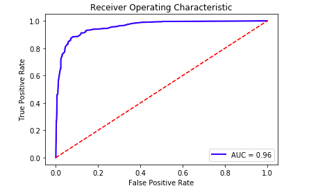
We could see the results are pretty good, here is the ROC curve I generated:
3. Summary
Random Forest uses decorrelated trees as base leaner and bagged them together to have a much higher accuracy and lower variance. The cost of bagging is that the tree model losses the interpretability.
Now we have an understanding of ensemble method. Let us talk about another ensemble method next time.