For the next four articles, I am going to review some basic but important topics such as Loss function, evaluation method, regularization and so on. After that I will move to review Deep learning and start to learn NLP.
Started from my first machine learning article, I have emphasized loss function's importance. So after covering most of basic ML models, it is time to summarize all these loss functions.
1. What is loss function
1.1 Definition
A loss function is a function that maps an event or values of one or more variables onto a real number intuitively representing some "cost" associated with the event. Basically, it is a measure of how good a prediction model does in terms of being able to predict the expected outcome. Thus it is very natural to always minimize a loss function for a machine learning model.
1.2 Terms Comparison
I believe you must have also seen some terms like Cost Function or Objective Function when you are reading some machine learning articles and books. But what are theirs differences comparing with loss function?
Basically, they are not very strict terms and highly related. However:
Loss function is usually a function defined on a data point, prediction and label, and measures the penalty. For example: * square loss \(l(f(x_i|\theta),y_i) = (f(x_i|\theta)-y_i)^2\)Cost function is usually more general. It might be a sum of loss functions over your training set plus some model complexity penalty (regularization). For example: * Mean Squared Error \(MSE(\theta) = \frac{1}{N}\sum_{i=1}^N(f(x_i|\theta)-y_i)^2\)
Objective function is the most general term for any function that you optimize during training. For example, when you perform MLE, the likelihood function will be the objective function you are going to maximize.
To make long story short, a loss function is a part of cost function which is a type of an objective function.
2. Different type of Loss Function
After understanding what is loss function, then let's talk about each of loss function one by one in detail. Generally speaking, Loss functions can be broadly categorized into 2 types: Regression Loss and Classification Loss.
2.1 Regression Loss Function
Regression model aims to return a continuous target value. Mathematically, a regression model can be formulated as: \[min_{f(x)}\sum_{I=1}^nl(y_i-f(x_i)) + R_{\lambda}(f)\] Where \(f(x_i)\) is the regression model, \(y_i-f(x_i)\) represents the deviation between \(f(x_i)\) and target value, \(l(r)\) represents a loss function that measures the loss generated by deviation, \(R_{\lambda}(f)\) is the regularization term for reducing the risk of overfitting.
2.1.1 Mean Squared Error/L2 Loss
- \(MSE = \frac{1}{n}\sum_{i=1}^{n}(y_i-f(x_i))^2\)
- Is the most common loss function for regression problem.
- Easy to calculate gradients
- Penalized heavily for far away values
2.1.2 Mean Absolute Error/L1 Loss
- \(MAE = \frac{1}{n}\sum_{i=1}^{n}|y_i-f(x_i)|\)
- Unlike MSE, MAE's derivatives are not continuous, and the gradient is large, making it inefficient and difficult to find the solution. (Can use dynamic learning rate)
- More robust to outlier since it does not use of square
2.1.3 Huber Loss/Smooth Mean Absolute Error
- \(L_{\delta}(y,f(x)) = \lbrace^{\frac{1}{2}(y-f(x))^2 \ \ for \ |y-f(x)|\le \delta}_{\delta|y-f(x)|-\frac{1}{2}\delta^2 \ \ otherwise}\)
- The combination of MAE and MSE to learn theirs advantages:
- Differentiable at 0
- Less sensitive to outlier
- \(\delta\) is the tuning parameter that determines what you're willing to consider as an outlier
2.1.4 Quantile Loss
- \(L_{\gamma}(y,f(x))= \sum_{I=f(x_i)<y_i}(\gamma -1)|f(x_i) - y_i| + \sum_{I=f(x_i) \ge y_i}(\gamma)|f(x_i) - y_i|\) where \(\gamma\) is the required quantile and has value between 0 and 1
- It is very obvious that \(\gamma\) controls which part of data we want to penalize on. If \(\gamma\) equals to 0.5, then quantile loss equals to MAE.
- From practical perspective, sometimes we want to know about the range of predictions as opposed to only point estimates
2.2 Classification Loss Function
Classification model aims to return a discrete value. A binary classification model can be formulated as: \[min_{f(x)}\sum_{I=1}^{n}l(y_if(x_i))+R_{\lambda}(f)\] Where \(y_i\) is the label of \(x_i\) and \(y_if(x_i)\) (margin) represents the deviation between \(f(x_i)\) and hyperplane. \(f(x_i)\) = 0 is the hyperplane.
The classification rule is that: with positive margin \(y_if(x_i)>0\), it is classified correctly; whereas margin \(y_if(x_i)<0\) means misclassified. The goal of the classification algorithm is to produce positive margins as frequently as possible.
2.2.1 0-1 Loss/Misclassification Error
\(\sum_{i=1}^{n}I(y_if(x_i)<0)\) or \(\sum_{i=1}^{n}I(y_i \neq f(x_i))\)
Non-convex, Non differentiable
Gives unit penalty for negative margin values, and no penalty at all for positive ones
2.2.2 Logistic loss/Binomial Deviance
From my previous post, Logloss is deduced by using the notation \(y\in\{0,1\}\). This is the most natural one cause it derives from Bernoulli probability model. But this notation make it hard for logloss to compare with other loss functions. Actually, logloss has another formula. This article has a very good explanation. Basically, by using notation \(y\in \{-1,1\}\), we integrate the label and the prediction together into the probability function. And then get the loss function by MLE.
- \(BD = log(1+e^{-y_if(x_i)})\)
- Differentiable
- Will always have loss
2.2.3 Cross Entropy Loss/Log Loss
Use the alternative label convention we get the logloss for Logistic Regression:
- \(Logloss = -y_iln(f(x_i))-(1-y)ln(1-f(x_i))\)
- Logloss is just the special case of Cross Entropy: -\(\sum_{j=1}^{c}p_j log p_j\) where j represent a class
- Gini index is another impurity measure close to Cross Entropy: Gini = \(\sum_{j=1}^{c}1 - p_j^2\) where j represent a class
- Related to information theory and multi-classification problem which I will cover later on
2.2.4 Exponential Loss
- \(Exp\ Loss = e^{-y_if(x_i)}\)
- Penalize incorrect predictions more and has a larger gradient
2.2.5 Hinge Loss
- \(Hinge = max\{1-y_if(x_i),0\}\)
- Convex, upper bound on 0-1 loss. Not differentiate at 1
- Only have 'margin error' when \(y_if(x_i)<1\)
Notice: Here I have only listed the loss function related to binary classification.
3. Loss Function Comparison
So after reviewing all these loss functions, I think we are able to see the differences among them. Basically, they have two major differences:
- Differentiable or not
- Robust to outlier or not
Then Let's compare them in detail.
3.1 Regression Loss Function Comparison
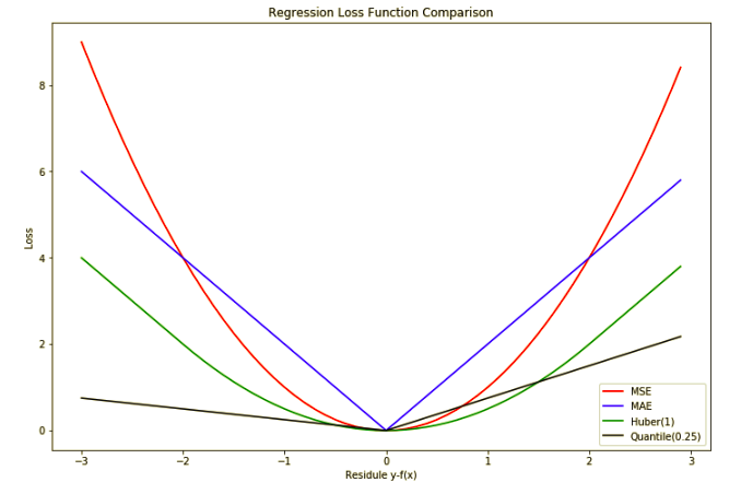
Above is the graph for comparing all the regression losses. Here are some summaries:
- MSE is sensitive to outliers but gives a stable and closed for solution
- MAE is useful for data is corrupted with outliers, but difficult to learn
- Huber Loss is the combination of MAE and MSE, but the choice of \(\delta\) is critical. And we need to tune this parameter which increase the computation cost.
- Quintile Loss is mainly used when you want an interval prediction. It is still mainly MAE, with different quantile value, it will decide to panelize on the upper bound value or lower bound.
3.2 Classification Loss Function Comparison
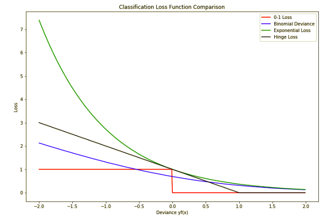
Here are the summaries for classification loss functions:
- 0-1 loss is not that sensitive to outlier since it gives unit penalty to all the misclassified data. But in another word, it is not sensitive to the data changes as well. So for tree growing model we may use other loss function like cross entropy.
- Both the exponential and deviance loss can be viewed as monotone continuous approximations
to misclassification loss. They continuously penalize increasingly negative margin values more heavily than they reward increasingly positive ones.
The difference between them is in degree. The penalty associated with binomial deviance increases linearly, whereas the exponential criterion increases the influence of such observations
exponentially. Not to say that exponential loss will be more sensitive to outliers.
3.3 Summary
- The loss function \(l(r)\) with an appropriate upper bound when \(r\) takes a large value is generally robust to the outliers.
- There is not a single loss function that works for all kind of data
Here is the link of Jupyter Notebook for loss function
Reference:
The Element of Statistical Learning
https://rohanvarma.me/Loss-Functions/
https://davidrosenberg.github.io/ml2015/docs/3a.loss-functions.pdf
An investigation for loss functions widely used in machine learning
https://heartbeat.fritz.ai/5-regression-loss-functions-all-machine-learners-should-know-4fb140e9d4b0
https://towardsdatascience.com/common-loss-functions-in-machine-learning-46af0ffc4d23