Now it's time to review machine learning knowledge. Actually, I was thinking about how to start reviewing this part a long time ago, but here is the dilemma: I have written some reviews before but it did not that useful as it is supposed to be. Therefore, I will follow these new rules as I'm writing the next several ML posts:
- Focus more on the mathematical theory of each model (MLE/Loss function/evaluation method)
- Pay attention to each model's assumption. Then I could list the pros and cons comparing with other similar models.
- For some basic but very important models (such as logistic regression/k-means/random forest), try to write the algorithm myself from scratch by Python.
All right, let us see whether it will be a good way to fully review the Machine Learning.
1. Introduction
Classification problem is one of the most important parts of supervised learning. In the next several posts, I will mainly cover these methods: Logistic Regression, Naive Bayes Model, Linear Discriminate Analysis(LDA), Quadratic Discriminate Analysis(QDA), KNN and SVM model.
In this post let us talk about Logistic Regression.
2. Theoretical Basis
Logistic Regression is a simple linear classification model. It seeks to model the probability that Y belongs to a particular category.
2.1 Logistic Regression Model
Logistic regression is a generalized linear model, there is no doubt that it has a very close relationship with the linear regression model. So let us then see how logistic regression model was generated, or how it extended from the linear regression model.
In a word, Logistic Regression model the class label given the data as:
$$P(y = k|x) = Bernoulli(p) = p^k\cdot (1-p)^{(1-k)}$$
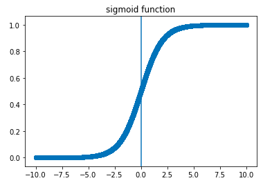
Then, what is $p$? It must have a relationship with our dataset $X$, we call it $p(X)$. From our first thought, can $p(X)$ be a linear regression model with $X$? However, we know $p(X)$ is a probability, and it could happen that for some $X$s, $p(X)$ could go out of $[0,1]$. So we need to find a function to both map $p(X)$ within $[0,1]$ and also catch the data's information. Then it comes sigmoid function.
$$\sigma(x) = \frac{1}{1+e^{-x}}$$
And here is the plot of this function:
Then our model is now like this:
$$P(y=1|x)= \frac{1}{1+e^{-\beta x}}$$
$$P(y=0|x)= \frac{e^{-\beta x}}{1+e^{-\beta x}}$$
Or more general:
$$P(y=k|x)=(\frac{1}{1+e^{-\beta x}})^k \cdot (\frac{e^{-\beta x}}{1+e^{-\beta x}})^{1-k}$$
where $\beta$ is a column vector. You may wonder where is the $\beta$ comes from. To see what the $\beta$ is, we need to do some transformation:
$$ln(\frac{P(y=1|x)}{P(y=0|x)}) = ln(\frac{1}{e^{-\beta x}})=ln(e^{x\beta})=x\beta$$
By looking at this formula, we could see how logistic regression connects with linear regression and what is $\beta$ function here:
- Control the weight of each predictor
- Also called scaling parameter: the larger the $\beta$, the closer the sigmoid function to indicator function
Finally, we often call this formula logit. If the logit larger than zero, we assign the data to class one; If smaller than zero, we assign the data to class two.
2.2 Parameter Estimation and Loss Function
Now we would like to estimate the coefficients $\beta$. We will use MLE here. Based on 2.1, we could easily write down the likelihood function (likelihood function is a function of the parameter of a statistics given data) of this model:
$$L(\mathbf{y},\mathbf{X}|\beta) = \prod_{i=1}^{n}L(y{_i},x_i|\beta) = \prod_{i=1}^{n}
(\frac{1}{1+e^{-x_i \beta}})^{y{_i}} \cdot (\frac{e^{-x_i \beta }}{1+e^{-x_i \beta}})^{1-y_i}$$
And the negative log likelihood is:
$$L(\beta)=-log(L(\mathbf{y},\mathbf{X}|\beta))=-\sum_{i=1}^{n}log(L(y{_i},x_i|\beta))=-\sum_{i=1}^{n}y_ilog(\sigma(x_i \beta))+(1-y_i)log(1-\sigma(x_i \beta))$$
Here we suppose each observation is independent with others.
Then:
$$\hat{\beta} = \arg\max_{\beta} L(\mathbf{y},\mathbf{X}|\beta)=\arg\max_{\beta}\prod_{i=1}^{n}L(y{_i},x_i|\beta)=\arg\min_{\beta}L(\beta)$$
So, it is natural that $L(\beta)$ is our loss function since we would like to minimize this if we want to get the optimal MLE. We often call this loss function: log loss.
Unfortunately, there is no explicit solution to this function, so we need to use some numerical algorithms such as gradient descent.
2.3 Model Assumption
After performing these analyses above, we could more easily understand the following assumptions:
- Require the observations to be independent of each other: That's the assumption for Bernoulli distribution
- Require little or no multicollinearity among the independent variables: Same with linear regression. Multicollinearity will influence mostly the interpretability and stability of the model. The estimate of one variable's impact on the dependent variable tends to be less precise (Since the weight of the parameter for logit can be used to explain the model); Also it produces large standard errors in the related independent variables and solutions that are wildly varying and possibly numerically unstable
- Assume linearity of independent variables and log odds: Since logistic regression provides a linear decision boundary ($\beta x = 0$), so if the linearity is not satisfied, it is impossiable to find a good solution.
- Require large sample size: always good to have more data
2.4 Multinomial Logistic Regression Model
Based on the analysis above, we find that logistic regression could solve the binary classification problem, then how to generalize the model to multi-classes condition?
1) As a set of independent binary regressions
One way to deal with this situation is to see this model as a set of independent binary regressions. So for $K$ possible outcomes, running $k-1$ independent binary logistic regression models, in which one outcome is chosen as a 'pivot' and then the other $K-1$ outcomes are seperately regressed against the pivot outcome. This would proceed as follows, if outcome $K$ is chosen as the pivot:
$$ln\frac{P(y_i=1)}{P(y_i=K)} =X_i \beta_1$$
$$\cdots \cdots$$
$$ln\frac{P(y_i=K-1)}{P(y_i=K)} = X_i\beta_{K-1}$$
If we exponentiate both sides, and solve for the probabilities, we got:
$$P(Y_i=1)=P(Y_i=K)e^{X_i\beta_1}$$
$$\cdots \cdots$$
$$P(Y_i=K-1)=P(Y_i=K)e^{X_i\beta_{K-1}}$$
Use the fact that all $K$ of the probabilities must sum to one, we find:
$$P(Y_i=K)=1-\sum_{k=1}^{K-1}P(Y_i=K)e^{X_i\beta_k }$$
$$=> \ P(Y_i=K)=\frac{1}{1+\sum_{k=1}^{K-1}e^{X_i\beta_k }}$$
Then we can use this to find other probabilities:
$$P(Y_i=1) = \frac{e^{X_i\beta_1}}{1+\sum_{k=1}^{K-1}e^{X_i\beta_k}} $$
$$\cdots \cdots$$
$$P(Y_i=K-1) = \frac{e^{X_i\beta_{K-1}}}{1+\sum_{k=1}^{K-1}e^{X_i\beta_k}} $$
2) As a log-linear model
The formulation of binary logistic regression as a log-linear model can be directly extended to multi-way regression. That is, we model the logarithm of the probability of seeing a given output using the linear predictor as well as an additional normalizaion factor, the logarithm of the partition function:
$$lnP(Y_i=1)=X_i\beta_1 - lnZ$$
$$\cdots \cdots$$
$$lnP(Y_i=K)=X_i\beta_K - lnZ$$
Since $\sum_{k=1}^{K}P(Y_i=K)=1$, therefore $Z = \sum_{k=1}^{K}e^{X_i\beta_k}$, then we have:
$$P(Y_i=c)=\frac{e^{X_i\beta_c}}{\sum_{k=1}^{K}e^{X_i\beta_k}}$$
The following function:
$$softmax(k,x_1,...,x_n)=\frac{e^{x_k}}{\sum_{i=1}^{n}e^{x_i}}$$is referred to as the softmax function. The reason is that the effect of exponentiating the values $x_1,...,x_n$ is to exaggerate the differences between them. As a result, softmax will return a value close to 0 whenever $x_k$ is significantly less than the maximum of all the values, and will return a value close to 1 when applied to the maximum value. Thus the softmax function can be used to construct a weighted average that behaves as a smooth function and which approximates the indicator function. Thus, we can write the probability equations as:
$$P(Y_i=c)=softmax(c, X_i\beta_1, ..., X_i\beta_K)$$
The softmax function thus serves as the equivalent of the sigmoid function in binary logistic regression.
3. Model Construction
Then let me construct a binary logistic regression from scratch by Python.
Due to the space constraint, please refer to this link to see more detailed coding information:
Jupyter Notebook For Logistic Regression
We could see logistic regression classify IRIS data very well.
4. Summary
Finally, lets summarize the pros and cons of logistic regression:
Pros:
- Outputs have a nice probabilistic interpretation. We can also find the important feature by looking at the parameter weights
- Outputs are easy to be modified based on the cut off threshold. Since LR output the probability score.
- Very fast and computationally cheap
- Can be regularized
Cons:
- Underperform when there are multiple or non-linear decision boundaries. It is not flexible enough to naturally capture more complex relationship
- Cannot handle large number of categorical features
- Cannot deal with the imbalanced data problem
If we want to use one sentence to describe logistic regression: Logistic regression assumes the binary data belongs to Bernoulli distribution, by using sigmoid function to approximate p(x), we then use MLE to estimate the parameter, and to get the solution we use gradient descent.
All right, I think now we could have a very good understanding of Logistic Regression both on theory and implementation. Let us move to some other classification problems in the next post.
Reference:
http://ml-cheatsheet.readthedocs.io/en/latest/logistic_regression.html
James的blog