RNN was designed for dealing with sequence data problem. For the next several articles, let's talk about that and finish the reviewing of deep learning basic knowledge.
1. Intro to RNN
1.1 Why we need it
Inputs and outputs length can be different: Remember CNN and RNN can only accept a fixed-size vector as input and produce a fixed-size output. But RNN can have different length of input and output:
Recurrent nets allow us to operate over sequences of vectors. In another word, it will share features learned across different positions of the input and allow information to flow from one step to the next.
1.2 The problem it can solve
RNN has been widely used recently due to the large volume of sequence data in real life. In general, here are the fields that RNN is used frequently:
- NLP: including sentiment analysis, language model, machine translation; speech recognition; image captioning
- Time-series processing including stock price prediction
2. RNN
2.1 RNN Structure
In order to solve the problem that normal FNN cannot remember the order and use previous information, we simply add a 'time axis' in the network structure that can pass prior information forward. That’s essentially what a recurrent neural network does:
Where each time we only pass one feature of a sample and move it forward with order.Mathematically: \[A_t = g(\omega_{aa}A_{t-1} +\omega_{ax}X_{t} + b_a)\] Which contains this layer's hidden unit information. We see it uses not only the new input \(X_{t}\) but also last hidden unit information \(A_{t-1}\). Here activation function \(g(x)\) normally will be tanh or relu.
Then if we output this layer's information: \[h_t = g(\omega_{ya} A_{t} + b_y)\] Here normally we will choose sigmoid function as \(g(x)\)
2.2 Limitation of RNN
2.2.1 Vanishing Gradient
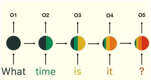
RNN unit is good for sequence data predictions but suffer from short-term memory. I found a very good illustration from Michael Nguyen's blog :

Suppose we have already trained a RNN with large corpus, and we want it to work as a chatbot that answers the question people has asked. Technically we will take the final output and pass it to the feed-forward layer to classify an intent. We can tell from the last recurrent unit's distribution that it hardly uses information from words 'what' and 'time', and mainly uses information 'is is ?' to make the prediction. Thus it is very natural to have a bad prediction output. That's what we called short-term memory. Why that happens? -- vanishing gradient problem again.
When doing back propagation, each node in a layer calculates it’s gradient with respect to the effects of the gradients, in the layer before it. So if the adjustments to the layers before it is small, then adjustments to the current layer will be even smaller. That causes gradients to exponentially shrink as it back propagates down. The earlier layers fail to do any learning as the internal weights are barely being adjusted due to extremely small gradients. And that’s the vanishing gradient problem.
Actually we can see that the lots of improvement in deep learning field is due to the success of solving the vanishing gradient problem. For RNN, LSTM and GRU were created as a method to mitigate short-term memory problem.
2.2.2 One direction information
Another limitation of RNN is that the prediction at a certain time only uses inputs earlier in the sequence but not information later in the sequence. To solve that problem, we will use bi-directional RNN.
3. LSTM
Both LSTM and GRU were created to solve the gradient vanishing problem by using a mechanism called gates. Gates are normal neural networks that regulate the flow of information being passed from one time step to the next. Let's look at LSTM step by step.
3.1 Cell State
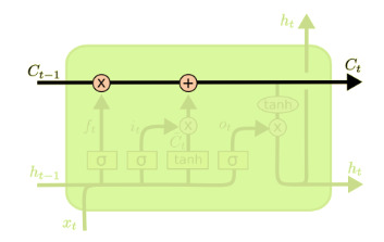
Cell State is the key to LSTMs. It runs straight down the entire chain, with only some minor linear interactions. It’s very easy for information to just flow along it unchanged,which is the reason it can refrain from vanishing gradient. I think the logic is kind of similar to Residual CNN: we make this layer similar with previous one if there is no learning, which indirectly shallows the network and helps with vanishing gradient.
3.2 Forget Gate
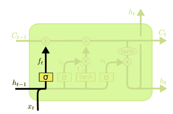
The first step in our LSTM is to decide what information we’re going to throw away from the cell state, and we use sigmoid function to decide that: (sigmoid function output value from 0-1 for each feature, after element-wise multiplication, we will get the final output) \[f_t=\sigma(\omega_f[h_{t-1},x_t]+b_f)\]
3.3 Update Gate
The next step is to decide what information we want to keep in the cell state. Same with forget gate, we use sigmoid function to decide. After that it will multiply with the new candidate value \(\tilde{C_t}\). \[\tilde{C_t} = tanh(\omega_c[h_{t-1},x_t]+b_i)\] \[i_t = \sigma(\omega_i[h_{t-1},x_t]+b_i)\]
Then it’s now the time to update the old cell state, \(C_{t-1}\), into the new cell state \(C_t\) by using forget and update gate's information: \[C_{t} = f_t * C_{t-1} + i_t * \tilde{C_t}\]
3.4 Output Gate
Finally we need to decide what we are going to output in the cell state by using output gate: \[o_t = \sigma(\omega_o[h_{t-1},x_t]+b_o)\] \[h_{t} = o_t * tanh(C_t)\]
4. GRU
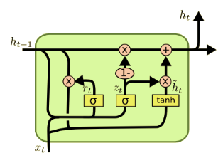
GRU is the simplified version of LSTM, it combines the forget and update gate together and also without using the memory unit(the cell state). Thus it is computationally faster. Mathematically: \[z_t = \sigma(\omega_z[h_{t-1},x_t]+b_z)\] Which works as update gate similar to what we have in LSTM \[r_t = \sigma(\omega_r[h_{t-1},x_t]+b_r)\] Which called reset gate that decides how much past information to forget. \[\tilde{h_t} = tanh(\omega[r_t * h_{t-1},x_t]+b)\] \[h_t = z_t * \tilde{h_t} + (1-z_t)* h_{t-1} \]
Reference:
DeepLearning.ai
https://www.youtube.com/watch?v=8HyCNIVRbSU http://karpathy.github.io/2015/05/21/rnn-effectiveness/ http://colah.github.io/posts/2015-08-Understanding-LSTMs/


