I have finished the course Deeplearning.ai long time ago but haven't summarized what I have learned before. Recently I realized that lots of knowledge can be easily forgotten if you will not use them very often. Thus one of the best way is to write them down in order to help you recap everything later on.
For this deep learning review series, I am planing to divide it into four articles:
- Basic Neural Network Structure
- How to improve Neural Networks
- Convolutional Neural Network (CNN)
- Recurrent Neural Network (RNN)
One notebook will be attached that tries to construct the network using the knowledge from each of the article.
Without further ado, let's start to look at the basic Neural Network Structure.
1. Introduction to Neural Network
Deep learning is a class of machine learning algorithms that:(From wikipedia)
- Use a cascade of multiple layers of nonlinear processing units for feature extraction and transformation.
- learn in supervised (e.g., classification) and/or unsupervised (e.g., pattern analysis) manners.
- learn multiple levels of representations that correspond to different levels of abstraction
From my point of view, one of the important breakthrough of deep learning is that it overcomes the challenge of the often tedious feature engineering task and helps with parameterizing traditional neural networks with many layers.
2. Neural Network Structure
2.1 Basic units
The basic unit of a neural network is the neuron, often called a node or unit. It receives input from some other nodes, or from an external source and computes an output. Each input has an associated weight \(\omega\), which is assigned on the basis of its relative importance to other inputs. The node applies a activation function \(g(z)\) to the weighted sum of its inputs as shown in Figure below:
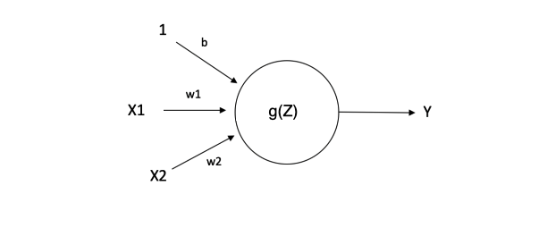
In summary:
- \(Z\) controls the linear transformation of the inputs
- \(g(Z)\) controls the nonlinear transformation of the inputs
So we could see that even for a unit it tries to use both linear and non-linear transformation to grab the information from the input data. So no need to say why a deep neural network with hundreds of unit can have very good prediction performance.
2.2 Feedforward Neural Networks
Then let's see a complete feedforward neural networks. It contains multiple neurons (nodes) arranged in layers. Nodes from adjacent layers have connections or edges between them. All these connections have weights associated with them. Let me make a specific example to further explain it:
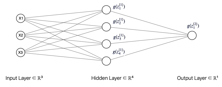
This is a feedforward NN with two layers (one hidden layer; one output layer). Input layer is not counted when calculating the total layers of one NN.
Since each NN will have lots of nodes and parameters. So it is very important to vectorize it. Here is the notation and dimension for each of the component of this NN:(suppose we have \(n\) sample data) \[X = [x^{(1)}, x^{(2)},x^{(3)}]_{(n,3)}\] Where \(x^{(i)}_{(n,1)}\) is the column vector contains all \(n\) samples' value for feature \(i\). \[Z^{[1]}_{(n,4)}=Z^{[0]}_{(n,3)}\omega^{[1]}_{(3,4)} + b^{[1]}_{(1,4)}\] \[g(Z^{[1]})_{(n,4)}=g(Z^{[0]}_{(n,3)}\omega^{[1]}_{(3,4)} + b^{[1]}_{(1,4)})\] Where \([i]\) tells us which layer does this variable belongs to; \((n,m)\) tells us the dimension for that variable
So the intuition to quickly come up with the dimension for the weights \(\omega\) is that weights are the connections to quantify last layer's influence to this new layer. So \(w_i^{[1]}\) should be a column vector with the number of rows equaling to the number of features from last layer. Then to stack all the \(\omega^{[1]}\) from this new layer, we get its dimension (#of nodes in last layer, # of nodes in this layer). For \(Z^{[i]}\) it is more easy to get its dimension. Since we can always think it as the input, its dimension will be like (# of samples, # of features(nodes) in this layer)
Finally: \[Z^{[2]}_{(n,1)}=Z^{[1]}_{(n,4)}\omega^{[2]}_{(4,1)}+b^{[2]}_{(1,1)}\] \[g(Z^{[2]}_{(n,1)})=g(Z^{[1]}_{(n,4)}\omega^{[2]}_{(4,1)}+b^{[2]}_{(1,1)})\]
2.3 Forward and Backward Propagation
- Forward propagation propagates the inputs forward through the network. The whole process above is just the example of forward propagation.
- Backward propagation propagates from the output to input. After forward propagation, we can choose one loss function to evaluate the output. Then each parameter can be updated by using gradient decent to minimize the loss.
3. Activation Functions
Activation functions are just functions that you use to get the output of a node. It calculates a “weighted sum” of its input, adds a bias and then decides whether it should be “fired” or not.
3.1 Why we need it
Activation functions normally have two properties:
- Non-linear
- Having activations bound in a range, say \((0,1)\) or \((-1,1)\)
The reason it has these two properties can help us understand why we need it:
- Each node is simply a weighted sum of inputs (linear), and activation function can add non-linearity to the model
- Mapping the bound to a range can make clear distinctions on prediction
3.2 Different Type of AF
3.2.1 Tanh Function
\[A = \frac{e^{z}-e^{-z}}{e^{z}+e^{-z}}\]
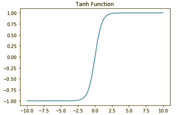
- Pros: similar to sigmoid but derivatives are steeper, bound to range (-1,1) so won't blow up the activations. Centering data can make the learning of next layer simple.
- Cons: when z values are large, gradient is very small and then learning speed is very slow => gradient vanishing
3.2.2 Relu Function
\[A = max(0,z)\]
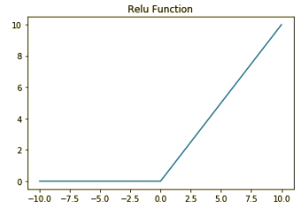
- Pros: Sparse activation: all inputs smaller than zero will be firing and the network is lighter. Also, relu is a good approximator. Any function can be approximated with combinations of ReLu
- Cons: It is not bound. The range of ReLu is \([0, inf)\). This means it can blow up the activation. Also, it faced with dying relu problem, which means for activation smaller than zero, gradient will be zero and the parameter will not be updated any more. To solve this problem, we introduce leaky Relu
3.2.3 Leaky Relu
\[A = max(0.01z, z)\]
Basically it just make it a slightly inclined line rather than horizontal line when z < 0.
4. Steps to construct a DNN
- Make sure the layers' dimension to initialize weights
- Forward propagation including linear forward and activation forward
- Define cost function
- Backward propagation
- Update parameter
- Make final prediction
Finally let's create a feed forward Neural Network by using Tensorflow.
Reference:
DeepLearning.ai
https://ujjwalkarn.me/2016/08/09/quick-intro-neural-networks/
https://medium.com/the-theory-of-everything/understanding-activation-functions-in-neural-networks-9491262884e0