From last article, we have talked about the relationship between SVM and logistic regression; What optimization problem SVM wants to solve and how it is solved. However, all these results are under one premise: our data needs to be linearly separable. But in fact, this condition is very hard to be satisfied. So in today's article let us talk about how SVM deals with linearly inseparable data.
1. Kernel Trick
It can be said that it is because kernel trick that makes SVM a very flexible and popular algorithm. And also, kernel trick is the most confusing part when I first tried to understand SVM. So what is kernel trick and what does it do?
1.1 Linearly Inseparable Condition
To explain that, we need to go back to our original problem a little bit: we want to use SVM to deal with linearly inseparable data.
One solution is that we can map our original feature space to a higher dimensional space. If you know SVM a little bit, you must have seen this intuitive picture before:
So even if we cannot find a hyperplane perfectly classify this data in original feature space, after the mapping to three dimensional space, we can easily find that perfect hyperplane. Basically, that is the idea how SVM solve this issue. But the question is: how to do this mapping?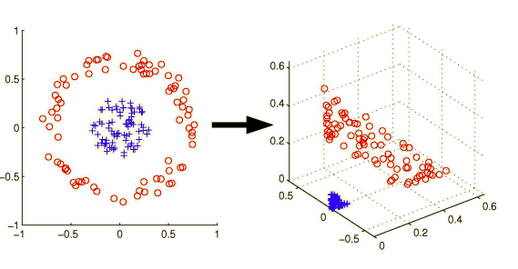
The most natural thought is to:
Find a nonlinear mapping function \(\phi(x)\): \(\phi: \chi \to \digamma \) where \(\digamma\) is a higher feature space than \(\chi\). Then use this function to map our data.
Use SVM to find appropriate hyperplane in our new feature space: \[f(x) = \sum_{I=1}^{n}\alpha_i y_i \langle \phi (x_i),\phi(x) \rangle\] (remember our most important results from the last article?)
Awesome! It seems that our problem has been perfectly solved. However, actually it can face with big problems: The mapping cost is very heavy. If we want to map our feature space into a very high dimension, both the mapping and the later calculation will be computational expensive.
Here comes our hero: The Kernel Trick.
1.2 Kernel Trick
Here is a very good example to illustrate how kernel trick solves this problem:
- Suppose \(X \ (x_1,x_2)\) is a test data point in a two dimensional space.
- We want to map it to a 6-dimensional space by using this mapping function: \[\phi(x) = (\sqrt{2}x_1, x_1^2,\sqrt{2}x_2,x_2^2,\sqrt{2}x_1x_2,1)\]
- Suppose one of our training data \(X_p\) is \((x_{p1},x_{p2})\)
So, first, if we use our previous method to finish this mapping, here is what we will do:
- Calculate \(\phi(X) = (\sqrt{2}x_1, x_1^2,\sqrt{2}x_2,x_2^2,\sqrt{2}x_1x_2,1)\)
- Calculate \(\phi(X_p) = (\sqrt{2}x_{p1}, x_{p1}^2,\sqrt{2}x_{p2},x_{p2}^2,\sqrt{2}x_{p1}x_{p2},1)\)
- Calculate \(\langle \phi (x_i),\phi(x) \rangle = 2x_1x_{p1}+x_1^2x_{p1}^2+2x_2x_{p2}+x_2^2x_{p2}^2+2x_1x_2x_{p1}x_{p2}+1\)
But what kernel trick does is that we find: \((\langle X,X_P \rangle +1)^2 = 2x_1x_{p1}+x_1^2x_{p1}^2+2x_2x_{p2}+x_2^2x_{p2}^2+2x_1x_2x_{p1}x_{p2}+1\) has the exactly same results but without really mapping our data into the high dimensional space!. \((\langle X,X_P \rangle +1)^2\) is called Kernel Function. Here is the definition from Wikipedia: Kernel Functions enable them to operate in a high-dimensional, implicit feature space without ever computing the coordinates of the data in that space, but rather by simply computing the inner products between the images of all pairs of data in the feature space.
So, in a word, kernel function can simplify the inner product calculation for feature space mapping and the coincidence is that the determinant part of SVM is decided by inner product! That is why kernel trick can be used in SVM conveniently and successfully!
1.3 Some Kernel Functions
- Polynomial kernels: \(k(x_1, x_2) = (\langle x_1,x_2 \rangle+R)^d\). It equals to map our data to a \(C_{m+d}^{d}\) space, where m is out original dimension.
- Gaussian kernels \(k(x_1, x_2) = exp(−||x_1 − x_2||^2/2\sigma^2)\) for \(\sigma >0\). It can map the data to and infinite dimensional feature space. So here \(\sigma\) is one of the hyperparameter that we need to tune for a better kernel.
2. Slack Variable
After being aware of kernel trick, we then move our model even further a little: how about our data cannot be separated perfectly by a (generalized) hyperplane even in a high dimension?
This could definitely happen when our outlier works as support vectors. To solve this problem, we introduce slack variable.
The idea for slack variable is that we allow some of the points come through our decision boundary and even pass through the hyperplane. And the variable which controls the allowable deviation from the hyperplane is called Slack Variable. Normally, we use \(\epsilon\) to represent it.
Here is the new optimization problem we want to solve after introducing slack variable: \[min \frac{1}{2}||w||^2 + C\sum_{i=1}^n \epsilon_i\] \[s.t. \ y_i(w^Tx_i+b)\ge 1-\epsilon_i,\ for \ \epsilon_i \ge 0, i=1,...,n\] To explain it a little bit, \(min\frac{1}{2}||w||^2\) is for maximizing the margin; \(min \ C\sum_{i=1}^n \epsilon_i\) is for controlling \(\epsilon_i\) not to be so large, since in that case all data points can pass through the decision boundary. C is a hyperparameter we need to tune. If \(C \rightarrow +\infty\), then \(\epsilon_i \rightarrow 0\), no data is allowed to pass the boundary; Or if \(C \rightarrow 0\), \(\epsilon_i \rightarrow +\infty\), every data is allowed to pass through the boundary.
The solution for this optimization problem is quite similar to the original one. The only difference is that we have a upper limit for the dual variable \(\alpha\) this time. So, we can still use kernel trick into our algorithm.
3. Cost Function
It seems abnormal that I put cost function at the end of talking an ML algorithm. The reason is that before introducing slack variable, we assume all our cases can be separated completely, in other words, there is even no loss in our model. Seems ridiculous right? but from learning SVM we then have a good idea about how one mutual ML algorithm develops from being full of loopholes to adapting for most conditions.
Let us re-look at our optimization problem: \[min \frac{1}{2}||w||^2 + C\sum_{i=1}^n \epsilon_i\] \[s.t. \ y_i(w^Tx_i+b)\ge 1-\epsilon_i,\ for \ \epsilon_i \ge 0, i=1,...,n\] The constraint \(y_i(w^Tx_i+b)\ge 1-\epsilon_i\) can be written more concisely as \(y_if(x_i) \ge 1-\epsilon_i\), Which, together with \(\epsilon \ge 0\), is equivalent to: \[\epsilon_i = max(0, 1-y_if(x_i))\]
Hence the learning problem is equivalent to the unconstrained optimization problem over \(w\): \[min\frac{1}{2}||w||^2 + C\sum_{i=1}^{n}max(0, 1-y_if(x_i))\]
So this function is the cost function for SVM. It consists of two parts:
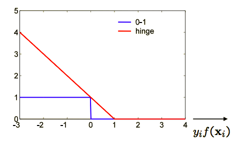
- The first part is \(max(0, 1-y_if(x_i))\) which is the loss function for SVM, and we call it Hinge Loss, here is what it looks like: So if we correctly classify the data, our loss is 0; but if we classify it falsely, the farther it is away from the boundary, the more loss we will get.
- The second part is \(\frac{1}{2}||w||^2\), which is the regularization term in the cost function. Minimizing the loss will always narrow the margin, so the regularization is required to prevent overfitting. This part tell us why SVM is called Structural Risk Minimization algorithm.
4.Model Implementation
To be continued...
5. Summary
Finally, let us make a brief summary.
- SVM tries to construct a hyperplane \(w^Tx+b =0\) to make classification
- we define maximal margin metric to decide the goodness of the hyperplane, then transform the original problem to a optimization problem
- By add Lagrange multiplier \(\alpha\), finding the solution of \(w\) and \(b\) equal to find the solution of \(\alpha\)
- In order to deal with linearly inseparable condition, we introduce kernel trick to map our data into high dimension but calculate still in a low dimension space
Reference:
An Introduction to Statistical Learning
https://people.eecs.berkeley.edu/~jordan/courses/281B-spring04/lectures/lec3.pdf http://www.eric-kim.net/eric-kim-net/posts/1/kernel_trick.html
http://www.robots.ox.ac.uk/~az/lectures/ml/lect2.pdf
http://www.robots.ox.ac.uk/~az/lectures/ml/lect3.pdf
https://www.zhihu.com/question/26768865/answer/34078149
https://blog.csdn.net/v_july_v/article/details/7624837