I am back again :D
I have just started my new job, so recently had little time to update my blog (Too Lazy…).
Here are the plans for my next several posts. First I will review SVM to finish the writing of fundamental ML algorithms part. Then I will move forward to deep learning.
All right, today let me talk about what is SVM. I decide to divide this topic into two posts: the first one aims to have an introduction about what is the relationship between SVM and Logistic Regression, what optimization problem it needs to solve; the second post will talk about kernel trick, slack variable and the loss function of SVM.
Need to notice that this time I will ignore introducing the basic concepts of SVM like hyperplane and margin.
1. Introduction
SVM is one of the most popular algorithms among decades. Even if its name is quite obscure, the idea behind it is quite easy to understand. Essentially, we aim to find a good classifier that maximizes the margin.
1.1 Relationship with Logistic Regression
Based on our previous post, we know logistic regression uses sigmoid function to map feature combination to \((0,1)\) and we can use logit to decide which class the new data point belongs to: \[ln(\frac{P(y=1|X)}{P(y=0|X)}) = ln(\frac{1}{e^{-\theta^T X}})=ln(e^{\theta^TX})=\theta^TX\] If \(\theta^TX>0\), we assign \(y=1\), otherwise we assign \(y = 0\).
Let me do some transformation about the logit: \[\theta^Tx_i = \theta_0+\theta_1x_{i1}+\theta_2x_{i2}+\cdots + \theta_px_{p1}\] We define \(\theta_0 = B\), \([\theta_1,\theta_2,\cdots,\theta_p ]=w^T\), then we have: \[\begin{align*} \theta^Tx_i &= \theta_0+\theta_1x_{i1}+\theta_2x_{i2}+\cdots + \theta_px_{p1} \\ &=B + w^Tx_i \end{align*}\] It is just the expression of a hyperplane. In the end, we just change the final mapping a little bit:
if \(B + w^Tx_i > 0\), we assign \(y = 1\); otherwise we assign \(y = -1\)
So, we can see that logistic regression and SVM use almost the same discriminant approach, and they both are linear classifier. So, not need to say sometimes they can obtain quite similar results. However, their differences are also very obvious, I will list here for now, hopefully we can understanding them clearly after reading this post.
- Loss function is different
- SVM only use SV to decide its decision boundary whereas LR will use all the data
- In most cases, SVM will use kernel trick but LR not.
- SVM need normalized data whereas LR doesn't need
- SVM has the function called Structural Risk Minimization (SRM) since its cost function contains regularization term. But LR's doesn't.
2. Model Structure
Next let us talk about the key part of SVM. Basically, the target of SVM is to find a hyperplane linearly separates two classes. Thus, to solve this problem, we need to figure out two things:
- How to define the goodness of a hyperplane
- How to find the best hyperplane based on the metric from question 1
2.1 Maximal Margine Metric
The most intuitional measure of the goodness of a hyperplane is to maximize the margin. But how to define it? Here, we use geometric margin as our distance measure. Suppose our hyperplane is \(w^Tx + b = 0\), then the geometric margin is: \[\hat{r} = \frac{y_p(w^Tx_p + b)}{||w||}\] To make it more clear, the distance between a point and a hyperplane has the fomular: \[dist = \frac{|w^Tx_i+b|}{||w||}\] Here we use \(y(w^T+b)\) to replace \(|w^T+b|\) because: \[if \ (w^T+b)>0 \ y=1 \\ if \ (w^T+b)<=0 \ y=-1\] so \(y(w^T+b)\) will always larger than or equal to zero, it not only gives us the distance between point and hyperplane, but also have some benefits when we introduce slack variable.
2.2 Optimization
2.2.1 Objective Function
After defining our metric, we can then summarize our goal as below in a more mathematic way: \[Max \ \hat{r} \\ s.t. \hat{r_i} \ge \hat{r} \ \ for \ i=1,..,n\] Where \[\hat{r_i} = \frac{y_i(w^Tx_i + b)}{||w||} \ge \frac{y_p(w^Tx_p + b)}{||w||}=\hat{r} \\=> y_i(w^Tx_i + b) \ge y_p(w^Tx_p + b)\] Here \(x_p\) represents the support vectors.
Since \((w^Tx + b)=0\) and \(c(w^Tx + b)=0\) define the same plane, so we have the freedom to choose the normalization of \(w\). In order for the convenience, we choose \(y_p(w^Tx_p + b)=1\), which means \(\hat{r}=\frac{1}{||w||}\). The following is a good illustration about this:
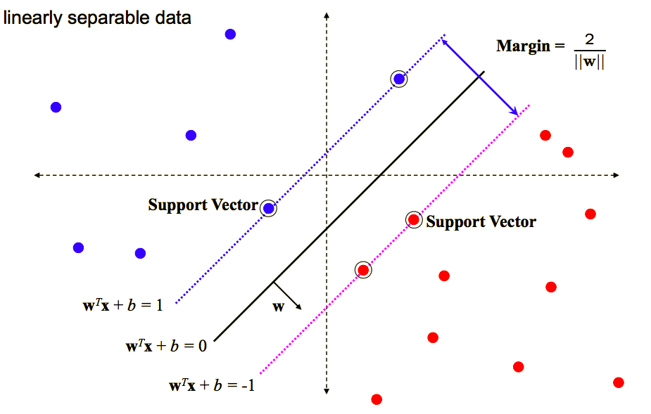
Then our optimization problem changes to: \[ Max \ \frac{1}{||w||} \\ s.t. y_i(w^Tx_i + b) \ge 1 \ \ for \ i=1,..,n \]
2.2.2 Optimization Method
After knowing our objective function, next we need to figure out how to solve this optimization problem. I will not have a whole mathematical proof here, but knowing the whole process is a necessity for better understanding what the kernel trick is.
Let us first further transform our objective function a little bit: \[ Min \ \frac{1}{2}||w||^2 \\ s.t. y_i(w^Tx_i + b) \ge 1 \ \ for \ i=1,..,n \] Which is equivalent to our previous objective function. Now our objective function is a quadratic function and at the same time the constraint is linear. The purpose is that we can then use Lagrange Duality and transform our problem to a dual problem.
I know it sounds very complicated, but basically, we add a Lagrange multiplier \(\alpha\) to our constraint and define the Lagrange function that describe our optimization problem by itself: \[L(w,b,\alpha)=\frac{1}{2}||w||^2-\sum_{i=1}^{n}\alpha_i(y_i(w^Tx_i + b)-1)\] And \[\theta(w)=max_{\alpha_i \ge 0}L(w,b,\alpha)=\lbrace^{\frac{1}{2}||w||^2 \ when \ y_i(w^Tx_i + b)-1 \ge 0} _{+ \infty \ when \ y_i(w^Tx_i + b)-1 < 0}\]
So our final objective function changes to: \[min_{w,b}\theta(w)\] I ignore all the steps for solving this optimization problem, and here are the results:
- \(w^{*} =\sum_{i=1}^{n}\alpha_iy_ix_i\)
- \(b^{*} = -\frac{max_{i,y_i=-1}w^{*T}x_i+min_{i,y_i=1}w^{*T}x_i}{2}\)
So, we substitute these optimal value into our original function: \[f(x) = (\sum_{i=1}^{n}\alpha_iy_ix_i)^Tx+b^* =\sum_{i=1}^{n}\alpha_iy_i\langle x_i,x \rangle + b^*\] Notice that \(x_i\) is our training data, and \(x\) is the new data point. Based on our previous discussion, if \(f(x) > 0\), then we will assign it to class 1. So we could see the only part that decides the classification result is \(\langle x_i,x \rangle\), the inner prodution. This finding is one of the most important result for SVM.
It can be said that the reason kernel trick is used easily in SVM is because of this result. So what kernel trick is? and how does SVM deals with data that cannot be classified perfectly? Let us see in the next post.
Reference:
An Introduction to Statistical Learning
http://www.robots.ox.ac.uk/~az/lectures/ml/lect2.pdf
http://www.robots.ox.ac.uk/~az/lectures/ml/lect3.pdf
支持向量机通俗导论 https://www.zhihu.com/question/26768865/answer/34078149