Now we have learned all the theories about MCMC. But how we can use it in practical? Especially how we can use it to solve Bayesian Inference problems?
1. Intuition
MCMC is a sampling technique but in most of the places it will be used for parameter estimation. How could this two connect with each other?
Actually that relates to the key concept from Bayesian framework: We treat unknown parameters as random, and they also follow some distributions. After knowing this, the connection is smoother: MCMC can be used to sample data from the parameters' distribution and then make an estimation. More specifically, this distribution is parameter's posterior distribution.
Here is the logic flow for one common scenario of using MCMC:
- We have gathered real life data from one distribution but we don’t know the parameter value of this distribution. So we want to estimate these parameters (The distribution is explicit even though we don't know the parameter)
- To estimate it, we want to sample data from these parameters' posterior distribution
- To sample from posterior equals to sample from unnormalized posterior (cause the evidence will be neutralized in MCMC)
- Using Bayes formula, to sample from unnormalized posterior we need to provide a prior
- Using MH or Gibbs sampling, we then need to either come up with a proposal distribution or provide the conditional distribution
2. Example - Estimation of Correlation
Suppose we are interested in modeling the correlation \(\rho\) between two streams of observations \((x_1,...,x_n)\) and \((y_1,...,y_n)\). And suppose we know the observations given the correlation belongs to Bivarite Gaussian distribution: \[p(x,y|\rho) \sim Normal(\mu,\Sigma)\] where \(\mu = [\mu_x,\mu_y]\) and \(\Sigma = \left(\begin{array}{cc} \sigma_{xx}&\rho \\ \rho & \sigma_{yy} \end{array}\right)\). For simplicity, we assume that we know \(\mu_x,\mu_y=0\) and \(\sigma_{xx},\sigma_{yy}=1\).
In this case, the likelihood function takes the following form: \[p(x,y|\rho) = \prod_{i=1}^{N}\frac{1}{2\pi\sqrt{1-\rho^2}}exp\{-\frac{1}{2(1-\rho^2)}[x_i^2-2\rho x_i y_i +y_i^2] \}\]
Next we need to specify a prior distribution for parameter \(\rho\). Suppose we also choose from normal distribution: \[p(\rho) \sim Normal(0,1)\]
Then using Bayes rule, we write the unnormalized posterior distribution for the correlation parameter \(\rho\) in the following ways: \[p(\rho|x,y) \propto \frac{1}{\sqrt{2\pi}}exp\{-\frac{\rho^2}{2} \}\prod_{i=1}^{N}\frac{1}{2\pi\sqrt{1-\rho^2}}exp\{-\frac{1}{2(1-\rho^2)}[x_i^2-2\rho x_i y_i +y_i^2] \}\]
Finally we try to find a symmetric proposal distribution. Here we choose a Uniform distribution centered at the current value of \(\rho\). \[\rho \sim Uniform(\rho^{i-1}-0.1,\rho^{i-1}+0.1)\]
Then the acceptance rate can be obtained using: \[\alpha(\rho^{i}|\rho^{i-1})= min\{1, \frac{p(\rho^i)}{p(\rho^{i-1})}\}\]
We are good to go for using Metropolis-Hastings Sampling, Python script can be found here: Notebook for MH-Sampling
Here are the results:
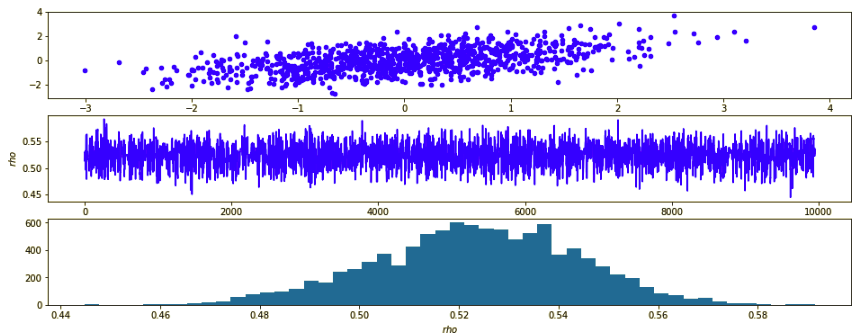
- Top image is what the real random data looks like which has the true correlation 0.5
- Middle row is the trace plot of \(\rho\) after burn-in, we can see the chain is almost stationary
- Bottom image plots the posterior distribution of \(\rho\) sampled from MCMC. The mean of this distribution is 0.52. So MCMC does give us a very good estimation.
3. Usage of Pymc3
For last example I didn't use specific MCMC package. Actually Pymc3 is a very good python package to perform MCMC and deal with other Bayesian Inference problem. I would like to use it more and get back to here later.
Reference:
http://www.mit.edu/~ilkery/papers/MetropolisHastingsSampling.pdf https://docs.pymc.io/notebooks/getting_started.html http://www.cnblogs.com/pinard/p/6645766.html http://people.duke.edu/~ccc14/sta-663-2016/16C_PyMC3.html http://www2.bcs.rochester.edu/sites/jacobslab/cheat_sheets.html