Recap: Now we understand both the theory and implementation algorithm for Metropolis-Hastings Sampling. But one limitations is that it is still not efficient when dealing with high dimensional distributions. So this article let's look at how Gibbs Sampling solves this problem.
1. Intuition
Let's look at the two-dimensional cases first. Suppose we have a known joint density function \(p(x,y)\). If we pick two data points with having the same \(x\) values: \(A(x_1,y_1)\), \(B(x_1,y_2)\), we find out that: \[p(x_1,y_1)p(y_2|x_1)=p(x_1)p(y_1|x_1)p(y_2|x_1)\] \[p(x_1,y_2)p(y_1|x_1)=p(x_1)p(y_2|x_1)p(y_1|x_1)\] In that case: \[p(x_1,y_1)p(y_2|x_1) = p(x_1,y_2)p(y_1|x_1)\] Which is: \[p(A)p(y_2|x_1) = p(B)p(y_1|x_1)\]
By combing with what we have learned from previous articles, we conclude that: For every two points on \(x = x_1\) this line, they will satisfy the Detailed Balance Stationary if we use \(p(y|x_1)\) as the transition matrix. Similarly, for two points with the same \(y\) values: \(A(x_1,y_1)\), \(C(x_2, y_1)\), they also satisfy this stationary: \[p(A)p(x_2|y_1) = p(c)p(x_1|y_1)\]
Therefore, we find a new way to get the transition matrix \(Q\) of target distribution \(p(x,y) = \pi(x,y)\): \[Q(A\to B) = p(y_B|x_1) \text{ if $x_A=x_B=x_1$}\] \[Q(A\to C) = p(x_C|y_1) \text{ if $y_A=y_c=y_1$}\] \[Q(A \to D) = 0 \text{ else}\] With this above construction of transition matrix \(Q\), we could easily see that for every two points \(x,y\), they will satisfy:
\[p(X)Q(x\to y) = p(y)Q(y \to x)\]
To visualize what I mean:
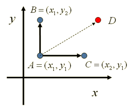
What an amazing finding!!
2. Gibbs Sampling Algorithm
- Input \(\pi(x_1,x_2,...,x_n)\) or all the conditional distribution; stationary threshold number \(n_1\), wanted sampling number \(n_2\):
- Initialize the sample \(x^{0}=(x_1^{0},x_2^{0},...,x_n^{0})\) from simple distribution
- For t = 0 to \(n_2+n_1-1\):
- Sample \(x_1^{t+1}\) from \(p(x_1|x_2^{t},x_3^{t},...,x_n^{t})\)
- Sample \(x_2^{t+1}\) from \(p(x_2|x_1^{t+1},x_3^{t},...,x_n^{t})\)
- ...
- Sample \(x_n^{t+1}\) from \(p(x_n|x_1^{t+1},x_2^{t+1},...,x_{n-1}^{t+1})\)
Then data points \(((x_1^{n_1},x_2^{n_1},...,x_{n}^{n_1}),..., (x_1^{n_1+n_2-1},x_2^{n_1+n_2-1},...,x_{n}^{n_1+n_2-1}))\) will be the samples from our targeted distribution \(\pi(x_1,x_2,...,x_n)\)
3. Summary
Gibbs Sampling is actually a special case of Metropolis-Hastings method where proposal distribution is the posterior conditions. So for Gibbs samplers we directly sample from the transition matrix \(P\) (the posterior conditions) and no need to think about acceptance criteria. It is commonly used in nowadays because we normally have high-dimensional data.
But the drawback is that the targeted distribution should be easy to calculate the conditional distributions.
Reference:
https://segmentfault.com/a/1190000012645418 http://www.mit.edu/~ilkery/papers/MetropolisHastingsSampling.pdf http://www.cnblogs.com/pinard/p/6645766.html