Let us continue our learning of generative classification methods. Recall that generative classification method aims to:
- Estimate joint probability $P(Y,X)$, and then use it to calculate $P(Y|X) = \frac{P(Y,X)}{\sum_i P(X|Y_i)P(Y_i)} = \frac{P(X|Y)P(Y)}{\sum_i P(X|Y_i)P(Y_i)}$
- Estimates not only probability of labels but also the features ($P(X|Y)$)
- Once model is fit, can be used to generate data
Last time, we talked about Naive Bayes Classifier, which gives us some basic understandings of Bayes classifier and generative model. Then This time let us talk about LDA and QDA.
1. Linear Discriminant Analysis (LDA)
1.1 Introduction
LDA assumes the class-conditional densities $P(X|Y=k)$ or $f_k(x)$ are Gaussian with a common covariance matrix so that:
$$P(X|Y=k) = f_k(x) = \frac{1}{(2\pi)^{(p/2)}|\Sigma|^{1/2}} e^{\frac{1}{2}(x-\mu_k)^T\Sigma^{-1}(x-\mu_k)}$$
And still $P(Y=k) = \pi_k= \frac{\# \ of \ observations \ in \ class\ k}{\# \ of\ observations}$
1.2 Parameter Estimation
Then we need to estimate the parameters of $f_k(x)$, we still use MLE here. I will ignore the mathmatical proof here since it basically is the MLE of multivariate normal distribution. Here is the results:
$$\hat \mu_k = \frac{1}{N_k}\sum_{i;Y=k}x_i$$
$$\hat \Sigma = \frac{1}{N-K}\sum_{k=1}^{K}\sum_{i;Y=k}(x_i-\hat \mu_k)(x_i-\hat \mu_k)^T$$
Here the estimated $\hat \Sigma$ is the unbiased estimation, and $N-K$ is the degree of freedom of this variable (Which we have talked during my inference's review).
1.3 Decision Boundary
After performing the first two steps, we could successfully calcualte $P(Y=k|X= x)$, then we can write the decision function as:
$$f(x) = \arg \max_k P(Y = k| X= x) = \arg \max_k \pi_k f_k(x)$$
so the corresponding decision boundaries are:
$$x: \pi_k f_k(x) = \pi_l f_l(x) \ \ k\neq l$$
then based on our estimation, we could simplify the above equation to: (I ignore the middle steps that contain absorbing everything that does not depend on k into a constant and take a logarithm)
$$log\pi_k - \frac{1}{2}\mu_k^{T}\Sigma^{-1}\mu_k + x^T\Sigma \mu_k=log\pi_l - \frac{1}{2}\mu_l^{T}\Sigma^{-1}\mu_l + x^T\Sigma \mu_l$$
And it is obvious that it is a linear equation in $x$. So LDA as its literal meaning is a linear classification method.
2. Quadratic Discriminant Analysis (QDA)
We know for LDA, the assumption that the inputs of every class have the same covariance $\Sigma$ can be quite restrictive; so in QDA, we allow each class has its own covariance matrix $\Sigma_k$
Then this time, we need to estimate the $\Sigma$ in every class, which is:
$$\hat \Sigma_k = \frac{1}{N-1}\sum_{i;Y=k}(x_i-\hat \mu_k)(x_i-\hat \mu_k)^T$$
And also our decision boundary will change since this time some terms related to $\Sigma$ cannot be neutralized. When we look back to our decision boundary, we get:
$$x: \pi_k f_k(x) = \pi_l f_l(x) \ \ k\neq l$$
$$log\pi_k - \frac{1}{2}\mu_k^{T}\Sigma_k^{-1}\mu_k + x^T\Sigma_k \mu_k-\frac{1}{2}x^T\Sigma_k^{-1}x - \frac{1}{2}log|\Sigma_k|= \\ log\pi_l - \frac{1}{2}\mu_l^{T}\Sigma_l^{-1}\mu_l + x^T\Sigma_l \mu_l-\frac{1}{2}x^T\Sigma_l^{-1}x - \frac{1}{2}log|\Sigma_l|$$
And it is obvious that the objective is now quadratic in $x$ and so are the decision boundaries.
3. KNN
3.1 Overview
After talking about using generative and discriminative classification method to approximate Bayes classifier. We then introduce a non-parametric method, called KNN.
KNN follows a very simple idea: Given a positive integer K and a test observation $x_0$, KNN identifies K points that are closest to $x_0$, represented by $N_0$ and then estimates the conditional probability that:
$$p(Y=j|X=x_0)=\frac{1}{K}\sum_{i \in N_0}I(y_i = j)$$
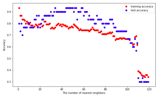
There is no doubt that $K$ has a drastic effect on KNN, actually, it controls the bias-variance trade-off of this model.
3.2 Model Implementation
Then let me construct KNN model from scratch. As normal, I will compare my result with sklearn.neighbors.KNeighborsClassifier in the end. Here is the plot of my model:

Here is the link of Jupyter Notebook For KNN.
4. Summary
Now I finish the review of generative classification methods. We could easily see the difference between these three models:
- LDA and QDA assume Gaussian density for $P(X|Y)$, but LDA needs the covariance for each class to be the same, and QDA does not.
- Naive Bayes assumes $P(X|Y) = \prod_j P(X_j|Y)$, which means each feature is conditional independent with other features under class y.
- KNN use distance-based learning to directly model $P(Y|X)$, it is effective to non-linear and complicated dataset but the computation is very costly.
Even though these four methods look simple, they do widely use in different fields. For example, Naive Bayes often works well when the data cannot support a more complex classifier such as text data classification and sentiment analysis.