Inference Review (Part2)

Let us continue our study and review of statistical inference. In this post, I will mainly talk about $\chi^2$ test and ANOVA test.

1. $\chi^2$ Test

1.1 Multinomial Distribution

Multinomial Distribution is an extension of Binomial distribution. It will have $n$ number of trials; $m$ number of conditions in each trial; $X_1,...,X_m$ is corresponding events; $\theta_1,...,\theta_m$ is the respective probabilities. the pdf is: $$p(X;\theta)=\frac{n!}{x_1!\cdots x_m!}\theta_1^{x_1}\cdots \theta_m^{x_m}$$

1.2 Goodness of Fit Test

Goodness of fit test examine how well does the data match what we think is true under $H_0$. Here is the basic set-up:

$$H_0: \theta_1=a_1,\theta_2=a_2,...,\theta_m=a_m$$ $$H_A: Otherwise$$ The test will be based on the following statistic: $$\chi^2=\sum_{i=1}^{m}\frac{x_i-E_{H_0}(x_i)}{E_{H_0}(x_i)}=\sum_{i=1}^{m}\frac{obs_i-n\cdot a_i}{n\cdot a_i} \sim \chi^2(m-1)$$ $x_i$ is the observed count in $i^{th}$ category

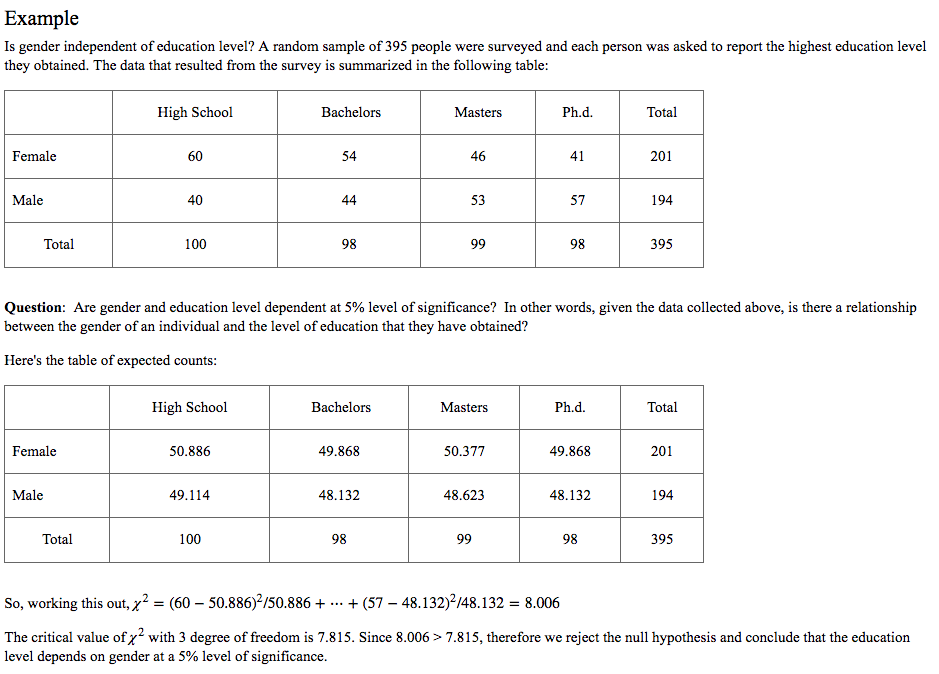
1.3 Test of Independence (Contingency Table)

This test aims to test whether two factors A, B are independent or not. Here is the basic set-up:

$$H_0: \theta_{i,j}=\theta_{i\cdot}\cdot \theta_{\cdot j},\ for\ all\ i,j$$ $$H_A: Otherwise$$ The test will be based on the following statistic: $$\chi^2=\sum_{i=1}^{r}\sum_{j=1}^{c} \frac{n_{ij}- \frac{n_{i.}n_{.j}}{n}}{\frac{n_{i.}n_{.j}}{n}} \sim \chi^2((r-1)(c-1))$$

Here is one good example I copy from Pennstate University's Website:

2. ANOVA Test

ANOVA test aims to test whether the mean value in different groups are the same or not. But essentially, it tests whether the factor has the effect to the numerical dependent variable.

2.1 Some definations and theories

First let us talk about some terminologies in ANOVA:

Factor is the object that we would like to test. And the different performance for this factor is called treatment. The data we get for each treatment are called observed value. For example, we want to test whether the complaint rate (observed value) is different in retail industry (treatment one), tourist industry (treatment two), household industry (treatment three). The factor here is industry.

Fundamental Theory
The reason that people call this test analysis of variance is because we will use variance to tell us whether there are significant mean differences among these groups. In other words, we need to analyze the source of the errors. What does that mean?

First of all, within one treatment, we have different observed values. Since we randomly sample the data, so there are only random errors here. This kind of error is called within-group error. It represents the degree of dispersion within each treatment.

Then, the observed values in different treatment are also different. These errors maybe result from the sampling random error, but may also result from the differences between these treatment (system error). These kind of error is called between-group error. It equals to the sum of random error and system error and it represents the degree of dispersion between these treatments.

Then the intuition for ANOVA is very clear: If the factor has no influence to our observed value, then there is only random error included in between-group error; then the averaged within-group error will be very similer to the averaged between-group error. Otherwise, there is system error in between-group error and it will larger than within-group error.

2.2 Assumptions for ANOVA

There are three basic assumption for ANOVA:

• Every treatment should belong to normal distribution
• The $\sigma^2$ for each treatment should be the same
• The observed value in one treatment is indepedent with other observed value in another treatment.

2.3 One-way analysis of variance

Here are the basic step for one-way analysis of variance.

1. Make Assumption: $$H_0:\mu_1=\mu_2=\cdots=\mu_k$$ $$H_1: \mu_i(i=1,2,...,k) \ not \ all \ equal$$
2. Construct Test Statistics:
   We need to calculate some important values first.
   1) sum of squares for factor A: (between-group square error) $$SSA = \sum_{i=1}^{k}n_i(\bar{x_i}-\bar{\bar{x}})^2$$ where $n_i$ is the number of observations in the $i^{th}$ treatment; $k$ is the number of treatment; $\bar{x_i}$ is the mean value in the $i^{th}$ treatment; $\bar{\bar{x}}$ is the mean value for all the observations.
   2) sum of squares for error: (within-group square error) $$SSE = \sum_{i=1}^{k} \sum_{j=1}^{n_i}(x_{ij}-\bar{x_i})^2$$ 3) sum of squres for total: $$SST = \sum_{i=1}^{k} \sum_{j=1}^{n_i}(x_{ij}-\bar{\bar{x}})^2 = SSA + SSE$$
   
3. Calculate Test Statistics:
   Since the size of error squares is decided by the number of observations, we then need average them first and then make comparison.
   1) Mean of squares for factor A: $$MSA=\frac{SSA}{df_{SSA}}=\frac{SSA}{k-1}$$
   2) Mean of squares error: $$MSE=\frac{SSE}{df_{SSE}}=\frac{SSE}{n-k}$$ If you want to know the reason why their degree of freedom should be like this, please refer to this link: https://www.zhihu.com/question/20983193
   In a word, it is because the mean value that let us lose some degree of freedom.
   
   Then, we obtain the F-statistics: $$F = \frac{MSA}{MSE}\sim F(k-1,n-k)$$ Based on our significane level, we then could make a conclusion. If $F> F_{\alpha}$, we then reject our null hypothesis.

2.4 Two-way analysis of variance

Since there are two factors in two-way analysis of variance, we need to know whether there is interaction effect for these two factors. If it has, we call it two-factor with replication; If not, we call it two-factor without replication

Normally, we will put one factor on the 'row' called row factor and another on the 'column' called column factor.

2.4.1 Two-factor without replication

Difference with the one-factor ANOVA:

1. Make two assumptions: one for row factor and one for column factor.
2. $SST=SSR+SSC+SSE$, where $SSR$ is the sum of squares for the row and $SSC$ is the sum of squares for the column. $SSE$ is still the random error.
3. Test two statistics $F_R=\frac{MSR}{MSE}\sim F(k-1,(k-1)(r-1))$, $F_C=\frac{MSC}{MSE}\sim F(r-1,(k-1)(r-1))$ individually.

2.4.2 Two-factor with replication

Difference with the two-factor without replication:
$SST = SSE+SSC+SSR+SSRC$, where $SSRC$ represent the sum of square for the interaction effect between row factor and column factor.

All right! I think now we've finished the review of statistical inference. It is time to play with Machine Learning! See you in the next post.