Last time we review the basic knowledge of Probability Theory, which gives us a fundamental understanding about statistics. This time we will go to the next step -- statistical inference.
Inference aims to learn about unknown quantities after observing some data that we believe contains relevant information. Normally, a statistical model specifies a joint distribution for observable random; parameters of that distribution are assumed unknown.
1. Parameter Estimation
1.1 Point Estimation
MLE (Maxmize Likelihood Estimation)
We want to find the MLE of $\theta$, $\hat{\theta}=g(x_1,...,x_n) s.t. L(\hat{\theta}) \ge L(\theta) $ for all other $\theta$.
The intuition here is that suppose we know the distribution of the sample data, we want to find the parameter that maximize the likelihood that we get these sample data.
MME (Method of Moments)
Compute moments such as $$E(X_i)=\mu, \quad E(X_i-\mu)^k$$, then equate sample moments to theoretical moments $$ \bar{X_n}=\mu, \quad \frac{1}{n}\sum(X_i-\bar{X})^k=E(X_i-\mu)^k $$
Bayes Estimator:
Let $L(\theta,\hat{\theta})$ be a loss function. $E_\pi(L(\theta,\hat{\theta}))$ is the bayes risk. An estimator $\hat{\theta} $is said to be a Bayes estimator if it minimizes the Bayes risk among all estimators.
Some notes on Bayes framework:
$$f(\theta|x_1,...,x_n) = \frac{f(x_1,...,x_n|\theta)h(\theta)}{f_x(x_1,...,x_n)}$$
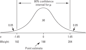
1.2 Interval Estimation
Some Important Distribution
- Chi-square distribution:
- t-distribution:
- F-distribution
Is a special gamma distribution when a = n/2 and b = 2; In particular, $$x_1,...x_n \sim ^{iid} N(0,1); then \sum_{i=1}^{n}x_i^{2}\sim x^{2}(n) $$
If $W\sim N(0,1)$ and $V\sim X^2(r)$ and $W\perp V$, then $$T=\frac{W}{\sqrt{V/r}}\sim t(r)$$
If $U\sim X^{2}(r_1)$, $V\sim X^2(r_2)$, and $U\perp V$, then $$F = \frac{U/r_1}{V/r_2}\sim F(r_1,r_2)$$
If $\bar{X} \sim N(\mu, \sigma^2/n)$, $\bar{X}\perp S^2$, then we have: $$\frac{(n-1)S^2}{\sigma^2}\sim X^2(n-1)$$ Based on the above two distributions, we could get: $$\frac{\bar{X}-\mu}{S}\sqrt{n} \sim t(n-1)$$ Quantiles of distribution
For any distribution, let $\alpha^{th}$ quantile (upper percentage point) be $$F(X_{\alpha})=P(X\le X_{\alpha}) = 1-\alpha$$ Confidence Interval
In statistics, a confidence interval (CI) is a type of interval estimate that is computed from the observed data. The confidence level is the frequency of possible confidence intervals that contain the true value of their corresponding parameter. The intuiation here is that we try to find a function $u(X, \theta)$ such that its distribution does not depend on $\theta$. Then we look for a,b s.t. $$P(a< U(X, \theta)< b)=1-\alpha$$ and finally invert this to get a statement about $\theta$ $$P(f_1(x;a,b))<\theta< P(f_2(x;a,b))$$
1.3 Important Interval Estimation Summary
1.3.1 Sample Mean
Let $X_1,...,X_n \sim N(\mu, \sigma^2)$
- $\sigma$ is Known:
- $\sigma$ is Unknown:
1.3.2 Sample Proportion
Let $X_1,..., X_n \sim Bernoulli(P)$, n kown, $Y = \sum X_i \sim Bin(n, p)$. We will use an approximation to construct a CI for p. Recall, by central-limit theorem: $$\frac{Y-np}{\sqrt{np(1-p)}}\sim N(0,1)$$then we have $$\frac{Y}{n}-Z_{\alpha/2} \sqrt{\frac{P(1-P)}{n}} < P<\frac{Y}{n}+Z_{\alpha/2} \sqrt{\frac{P(1-P)}{n}}$$ Here we need to use MLE to get the point estimation of $\hat{P}= \frac{Y}{n}$
1.3.3 Sample Variance
Let $X_1,...,X_n \sim N(\mu, \sigma^2)$, both $\mu$ and $\sigma$ are unknown. $$\frac{(n-1)S^2}{\sigma^2} \sim X^2(n-1)$$ Brief Summary: For sample mean and proportion, if our sample size is large or we know the $\mu$ and $\sigma$, we normally use z-statistics; If we do not know $\sigma$, we will use t-statistics. For sample variance, we use chi-square statistics.
2. Hypothesis Testing
Here is a basic set up for a hypothesis test: we have some default belief about a parameter, this is our null hypothesis. And we're trying to investigate whether an alternative hypothesis is in fact true.
2.1 Some definations and summary
Type I and II error
Upon conducting a test we will arrive at one of two possible conclusions:
| $H_0$ is True | $H_A$ is True | |
|---|---|---|
| Reject $H_0$ | Type I error | Correct |
| Not Reject $H_0$ | Correct | Type II error |
More specifically, Type I Error equals to $P(\theta \in C|H_0)$, which means when $H_0$ is true, the probability that our parameter locates in critical region (rejection region). Type II Error equals to $P(\theta \in C^c|H_A)$, which means when $H_A$ is true, the probability that our parameter locates in the non-rejection area.
Based on the analysis above, we could see an obvious trade-off between these two type of errors. Since if we shrink the rejection area to decrease type I error, the non-rejection area will be larger which means the type II error will increase. The reason that we always first control type I error is that:
In practical, our null hypothesis is always very specific, whereas the alternative hypothesis is always very general. For example, $H_0=1000$, then $H_A\ne 1000$. Therefore, in comparison, we are more willing to know the error that one specific hypothesis is actually false.Significance Level
In practice, we often specify the maximal allowable type I error. Specifically, $P(\theta \in C|H_0) \le \alpha$, where $\alpha$ is the significance level. In another word, it defines the probability of rejecting the null hypothesis when it is true.
P value
P value is the probability of observing a result equal to or more extreme than what was actually observed, when $H_0$ is true.
Intuition Here: We start by saying assume $H_0$ is true. We collect data, and analyze it in some manner. When we look at that summary, the p-value let us know how reasonable our data is, assuming the null is true. When the p-value is small, it tells us one of two things. 1) If the null hypothesis is true, then we’re seeing something that’s unlikely or 2) these data are really incompatible with the null hypothesis (because we had a low chance to see this or more extreme results), therefore, I suspect the null hypothesis does not hold. Your job is to pick an alpha level to decide your comfort in making a Type I error.
Example:
We want to construct a hypothesis test about whether this person is guilty or not. Suppose he is innocent, after observing some data, we find the probability that these resources appear is 4%. And our significance level is 0.05. Based on that, we could reject our null hypothesis.
In a word, we could see that the key idea behind Hypothesis Testing is that we think small probability event is not gonna happen easily. We will set a threshold (significnace level) to define the tolerance level for this small probability event; and p value will tell us the probability of obtaining at least as extreme as the one in our sample data, assuming the truth of the null hypothesis. After compare this p value with our significace value, we can then make a decision to accept or reject our hypothesis.
2.2 Constructing Hypothesis Tests
After understanding the whole process of hypothesis testing, we will then wonder how to choose the best critical region. Since it is the most important part of our test. In general, the best critical region of size $\alpha$ is that for every subset $A$ such that $P_{H_0}(x \in C) = \alpha$, we have $P_{H_A}(x \in C^c) \le P_{H_A}(x \in A^c)$. Which means we have minimum type II error with fixed type I error.
We have three method to find the best critical region:
Let us talk about other inference knowledge in the next post!